A recent batch of algorithm research results released by OpenAI has attracted attention. One claim is that integer multiplication can beat O(n log n) time. Yet researchers proved back in 1972 that integer multiplication requires at least Ω(n²) computational cost. Who got it wrong?
What does algorithmic complexity actually measure? Why can the same problem lead to such different conclusions? Through integer multiplication, matrix multiplication, and the FFT, this article examines the assumptions behind complexity results that are all too easily overlooked.

Author: silverxz
Reviewed by: emmm

On October 6, 2026, OpenAI released drafts of 722 papers, including important results in theoretical computer science—if verified as correct—and particularly some surprising complexity improvements for classical problems. However, many people reporting these results have oversimplified them. One such list reads:

…
No. 130: The FFT’s limit is not $O(n (\log n))$ ; it can reach $O(n (\log n)^{1 - \varepsilon})$ .
No. 109: Integer multiplication is not limited to $O(n (\log n))$ either; it can reach $O(n (\log n)^{1 - \varepsilon})$ .
…

Lists like this may help spread the news, but they do not help us understand what the results actually mean and may even be misleading. They pair a “problem” with a “complexity,” suggesting a potentially misleading relationship while leaving out an equally indispensable third element: the model of computation, which determines how complexity is measured. That is what this article aims to introduce and clarify. Before discussing an algorithm’s complexity, we must establish which computational model it uses. Staring at a big-O expression is not enough.

OpenAI’s unverified results happen to cover a wide range of computational models, so we can use them as examples while explaining what these models mean. A reminder, though: these results still await verification. This article does not discuss their specific techniques or correctness; we are only trying to understand the literal meaning of their claims.

This article offers something of an “advanced understanding” of algorithmic complexity. It assumes readers already have a basic grasp of complexity and are familiar with asymptotic notation such as $O,\Omega, \Theta, o$ . That calls for the knowledge of an early undergraduate computer science student or someone with experience in programming contests. If you are a little rusty, here are the definitions:

$\begin{aligned} f(n)=O(g(n))&\iff \exists c>0,\quad f(n)\le cg(n)\ \text{for all sufficiently large}\ n,\\ f(n)=\Omega(g(n))&\iff \exists c>0,\quad f(n)\ge cg(n)\ \text{for all sufficiently large}\ n,\\ f(n)=\Theta(g(n))&\iff f(n)=O(g(n))\ \text{and}\ f(n)=\Omega(g(n)),\\ f(n)=o(g(n))&\iff \forall c>0,\quad f(n)\le cg(n)\ \text{for all sufficiently large}\ n. \end{aligned}$

A starting example

Consider the following nested loop.

int sum = 0;
for (int i = 0; i < n; i++) {
    for (int j = 0; j < n; j++) {
        sum = sum + a[i][j];
    }
}

If you know a little about algorithmic complexity, one glance may be enough for you to say that this code “obviously” has complexity $O(n^2)$ .

But why?

Asked to break it down carefully, you might say that the code performs $n^2$ additions and $n^2$ assignments. Looking more closely, you might add that it also accesses a[i][j] in memory $n^2$ times. Since each of these operations costs $O(1)$ , the total is $3\cdot n^2 \cdot O(1) = O(n^2)$ .

Indeed, this is how we normally analyze algorithms. Addition, subtraction, multiplication, division, assignment, random memory access—we treat all these basic operations as $O(1)$ .

But that is not something we should take for granted. It is an explicit choice made to calculate an algorithm’s complexity. Once you choose to make those operations $O(1)$ , you can calculate the total complexity on that basis. The choice itself is neither right nor wrong, but different choices give different answers with different meanings.

To understand this, consider a multiplication version of the nested loop, this time in Python. Python integers have arbitrary precision: as long as memory permits, they can keep growing without overflowing.

def compute(n):
    product = 1
    for i in range(n):
        for j in range(n):
            product = product * 2
    return product

What is its complexity?

If a multiplication costs $O(1)$ —that is, if computing product * 2 costs $O(1)$ —then the total is still $O(n^2)$ . But if you actually run it, you will find that it behaves very differently from the previous nested loop. The intermediate result grows exponentially, and for large $n$ , multiplication gets very, very slow as that result expands. If you have implemented arbitrary-precision addition or multiplication yourself, you will understand why: the time these operations take depends on the number of digits. Assuming they always cost $O(1)$ no longer reflects actual performance.

You might say, “All right, I get it. You’re just saying it’s wrong to treat integer operations as $O(1)$ when the integers are huge. Obviously. That’s so simple—why bother explaining it?” Hold on: I did not say it was wrong. Remember what we said? What counts as $O(1)$ is a choice, and a choice is neutral, not absolutely right or wrong. What matters is whether it is the choice you want. If someone says, “Assuming multiplication costs $O(1)$ , the algorithm above has complexity $O(n^2)$ ,” that is entirely correct. It simply does not describe the performance of this Python code on a typical machine very well. You can say, “You’re right, but that isn’t the choice I want,” or, more bluntly, “Stop stating the obvious.” But the obvious statement is still true.

You may wonder why I am being so particular about the wording. The reason is that in theoretical computer science, the complexity of many problems admits more than one reasonable choice. None is absolutely correct; it depends on what you want. Integer multiplication and the FFT are both good examples. Let’s start with the former.

Integer multiplication and Turing machines

The abstract of OpenAI’s preprint Integer multiplication below n log n says:

We give a deterministic algorithm that multiplies two n-bit integers in $O(n(\lg n)^{1-\kappa})$ worst-case time, with $\kappa = 2^{-182}$ , on one fixed finite-alphabet Turing machine with a fixed finite number of one-dimensional tapes.
We give a deterministic algorithm for multiplying two n-bit integers in worst-case time $O(n(\lg n)^{1-\kappa})$ , where $\kappa = 2^{-182}$ , on a Turing machine with a fixed finite alphabet and a fixed finite number of one-dimensional tapes.

The bold text specifies the model of computation.

You do not need to know the details of a Turing machine. It is enough to know that it has one or more infinitely long one-dimensional tapes. “One-dimensional” means that the tapes consist of cells arranged in a row. The tapes serve as memory, and their cells as memory locations. Each tape has a movable read/write head that can read or write only the cell it currently occupies. To reach another cell, it must move there one cell at a time. In this model, moving a head by one cell or reading or writing one cell normally costs $O(1)$ . That is the model’s choice. Here is a schematic of a Turing machine.

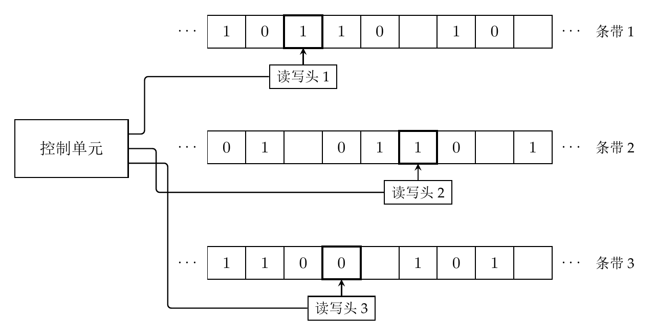
A multi-tape Turing machine: one control unit connects to three read/write heads, each assigned to a tape.

Notice that although tapes function as memory, reaching a distant cell requires moving the head one cell at a time. Unlike ordinary memory, they do not offer random access. Random access means an operation such as a[r], which uses a variable $r$ to address a memory location directly. A Turing machine cannot do this directly. If its head is at a[0], reaching a[r], $r$ cells away, requires $r$ head movements and costs $O(r)$ .

These low-level details have real consequences. A machine with multiple tapes has multiple heads, indirectly permitting more flexible memory access. OpenAI’s result is established on just such a multi-tape machine. If only one tape is allowed, together with an additional read-only input tape, Juan Bulnes proved a lower bound of $\Omega(n^2)$ in 1972.

If we discuss complexity without stating the chosen model and how operations are charged, looking only at asymptotic notation produces an absurd-looking contradiction: how can the same problem be both $O(n(\lg n)^{1-\kappa})$ and $\Omega(n^2)$ ? We now know that there is no contradiction. The models differ, and their only difference here is the number of tapes permitted. This illustrates that a small change in the computational model can make a major difference to complexity. That is the lesson I want this example to convey.

It also corrects some intuitions we may have as beginners. We might imagine that every problem has one unique, true “optimal complexity” waiting to be discovered. That is not how things work; the idea ignores the model. Omitting the model makes for better publicity: “Integer multiplication breaks $O(n\log n)$ !” sounds much more exciting and newsworthy than “Integer multiplication breaks $O(n\log n)$ on a multi-tape, finite-alphabet Turing machine.” But the latter is the actual claim. The seemingly wordy qualification is a substantive part of the result: it respects what was achieved without diminishing its real significance.

Beginners may also believe that a problem’s upper and lower bounds reflect some objective difficulty. In coarse-grained complexity analysis, this is true to an extent, since reasonable models can often be reduced to one another with polynomial overhead. A problem in P—one decidable in polynomial time—does not cease to be in P merely because the number of tapes changes. In that sense, classes such as P and PSPACE do capture something about these problems’ “intrinsic difficulty.” In fine-grained complexity, where every detail matters, however, upper and lower bounds are closely tied to the chosen model, as we have just seen.

You may have more questions: “Both of these Turing-machine models seem strange. Neither allows random access, so why use them?” Or, “Are there models closer to real machines?” For integer multiplication alone, finding a truly practical model is not easy, and a detailed discussion would become complicated. But if you simply want to know about other models, especially ones permitting random access, the answer is yes—there are plenty. Let’s turn to another problem.

Subset Sum and word-RAM

OpenAI has also attempted two contributions on Subset Sum. The problem is defined as follows: given $n$ positive integers $a_1, \dots, a_n$ and a positive target integer $t$ , can we select some of the numbers, without selecting any one twice, so that their sum is exactly $t$ ?

The preprint is titled Subset Sum in Time $O(2^{0.49 n})$ . We now know that looking only at $O(2^{0.49 n})$ is not enough: to understand the result, we must ask which model it uses. As with integer multiplication, let’s start with the abstract:

We give a uniform randomized classical algorithm for Subset Sum with bounded error and worst-case running time $O(2^{0.49n})$ on polynomial-bit inputs in a word-RAM model, where n is the number of input integers.
We give a uniform, classical randomized algorithm with bounded error for Subset Sum. When input bit lengths are polynomial in $n$ , its worst-case running time is $O(2^{0.49n})$ in a word-RAM model, where $n$ is the number of input integers.

This improves on the $2^{n/2}/poly(n)$ result of Chen–Jin–Randolph–Servedio 2023, reducing the exponent from $1/2$ to $0.49$ . The change looks tiny, but it is already a substantial breakthrough.

Here we encounter a new model: word-RAM. Its name means exactly what it says. RAM stands for random-access machine, so the model allows random memory access. “Word” means that operations act on words and are assumed to cost $O(1)$ .

Word-RAM is not a single model but a family of models. To specify one, we must state how many bits a word contains—the word length $w$ —and which $O(1)$ operations on words are permitted. The latter usually follows convention: reads, writes, addition, subtraction, and bitwise operations are allowed. The main disagreements concern whether multiplication, division with remainder, and modulo are $O(1)$ . Thus word length $w$ is the principal parameter, and we will now discuss how it is chosen.

Fixing $w=64$ would give something fairly close to the machines we commonly use. But in the most common word-RAM models, word length is not a fixed constant such as $w=64$ . It is variable, changing with input size. Generally, if the input size is $n$ , the word length satisfies $w=\Omega(\log n)$ . Why? A word can hold at most $2^w$ different addresses. If $w$ is constant, the memory addressable by one word is also constant. Addressing location $n$ would then require $\log n$ words just to store the address, which is awkward. Such a model can be considered, but the more common choice is simply to let $w$ grow with $\log n$ , ensuring that an address always fits in a single word. Notice that word length itself can be described asymptotically, since a constant factor does not change asymptotic complexity.

The resulting word-RAM model is more powerful than the Turing machine we discussed, because operations on words cost $O(1)$ . Adding two $\log n$ -bit integers therefore costs $O(1)$ on a word-RAM, while a Turing machine processing one bit at a time faces a lower bound of $\Omega(\log n)$ .

But why did we write $w=\Omega(\log n)$ instead of simply setting $w=\Theta(\log n)$ ? Because $w=\Omega(\log n)$ is usually only a basic addressing requirement. Particular problems may impose further requirements, making words longer. For example, in problems involving integers, we often want each integer to fit in a word, requiring the word to be at least as long as those integers.

For Subset Sum, let

$b =\left\lceil\log_2(1+\max\{t,a_1,\dots,a_n\})\right\rceil$

Thus $b$ is the maximum length of the $n+1$ input integers. For this problem, the word-RAM model usually also requires $w = \Omega(b)$ .

We have seen that word length and the permitted instruction set both affect a model’s power. What choices did OpenAI make? Even if such parameters are absent from the abstract, they should appear near the beginning. Indeed, the paper states at the outset that multiplication, division with remainder, and modulo are permitted, with word length

$w=\left\lceil4(n+b+\log(n+2))\right\rceil$

In other words, $w = \Theta(n+b)$ . That differs from what we just discussed: there is an extra $n$ . The analysis on pages 26–27 explains that this ensures all memory used during execution can be addressed by a single word. We can now say that we understand the model underlying the paper’s claimed result.

However, the previous state-of-the-art Subset Sum result, Chen–Jin–Randolph–Servedio 2023, assumed $w=\Theta(\log t)$ , essentially $w=\Theta(b)$ . Any $a_i$ larger than $t$ can be discarded, so we may assume $a_i \leq t$ , making $b$ and $\log t$ the same order. If $n$ cannot be absorbed into $b$ , these two word-RAM models are not equivalent! For example, when $b=o(n)$ , OpenAI’s model is more powerful than the one chosen by Chen–Jin–Randolph–Servedio 2023. They are no longer the same computational model. In that case, we could not claim that OpenAI had improved the earlier result, because the two could not be directly compared.

Fortunately, that mix-up has not actually occurred. For Subset Sum, the case $b<0.48 n$ is unimportant here. The classical knapsack algorithm runs in $O(nt)=O(n2^b)$ , so when $b<0.48 n$ , this simple algorithm already beats both OpenAI’s and Chen–Jin–Randolph–Servedio’s results. That case can be left to the knapsack algorithm and set aside in this discussion. We can therefore assume $b\geq 0.48 n = \Omega(n)$ , giving $w=\Theta(n+b) = \Theta(b)$ ; the models differ only by constants. Similar reasoning already appeared in Chen–Jin–Randolph–Servedio 2023, making this an established convention. If OpenAI’s result is verified, it is indeed a substantive improvement.

This example has introduced the word-RAM model and shown how to compare results: we must carefully compare the models used by the two results. Different models do not necessarily make results incomparable, but comparison must rest on careful analysis. That is this example’s lesson. We will see a similar analysis with the FFT.

To avoid a misunderstanding, studying Subset Sum on a word-RAM does not mean it “ought” to be studied there. We could instead charge by the bit, using a bit-cost RAM. A $b$ -bit integer would no longer be atomic; addition, multiplication, comparison, and other operations would be charged according to the number of bits actually processed. For the inputs considered here, where $b=\operatorname{poly}(n)$ , expanding a word operation into polynomially many bit operations introduces only a factor polynomial in $n+b$ . This can be absorbed into the polynomial factor of the paper’s stronger, more precise bound $T(n)=2^{0.489995n}\operatorname{poly}(n+b+2)$ . Using the assumption $b=\operatorname{poly}(n)$ then gives the same $O(2^{0.49n})$ bound, without affecting the essential improvement in the exponent to $0.49$ .

We could also study the problem on a Turing machine, paying extra for memory access. As we said earlier, the computational model is often a choice, not a matter of “this problem must have this one correct model.”

Matrix multiplication and arithmetic complexity

Our discussion of Turing machines and word-RAM may have made computational models sound like things neatly ranked from weaker to stronger. If so, I hope the next example clears up that impression.

OpenAI released a preprint on matrix multiplication, An Upper Bound of 9/4 for the Matrix Multiplication Exponent, with this abstract:

We prove that the exponent of matrix multiplication over the complex numbers is at most 9/4.
We prove that the matrix multiplication exponent over the complex field is at most 9/4.

Few words, an enormous claim. This is a major result, and signs in the paper suggest that $9/4$ may be only the starting point for the method. Of course, that still needs to be checked.

Unlike the previous two examples, OpenAI does not specify its computational model in this abstract. That is because this problem has a long-established default model. To explain it, we must first introduce the problem itself.

This problem is fundamentally different from those defined on a Turing machine or word-RAM. It can be described as follows. Given two $n\times n$ matrices $A=(a_{ij}), B=(b_{ij})$ with entries in the complex field $\mathbb{C}$ , compute every entry of $C=A\times B$ from the entries of $A, B$ and preselected complex constants, using complex addition, subtraction, and multiplication. What is the minimum number of complex arithmetic operations required? This definition treats all three operations as $O(1)$ .

That is only a rough description; the actual definition is somewhat more involved. We cannot allow special treatment for each individual pair of matrices $A, B$ . Otherwise, we could simply select the answers as complex constants and output them, which would be uninteresting. Strictly speaking, special treatment is allowed for each $n$ , but for the same $n$ , we must use the same constants and the same mechanical sequence of operations to produce the answer. This mechanical computation takes the form of a circuit diagram, or directed acyclic graph. “Circuit” here is terminology inherited from computational complexity, not a real physical circuit.

For instance, if we choose brute-force multiplication of $2\times 2$ matrices, we compute

$\begin{aligned} c_{11}&=a_{11}b_{11}+a_{12}b_{21},&c_{12}&=a_{11}b_{12}+a_{12}b_{22},\\ c_{21}&=a_{21}b_{11}+a_{22}b_{21},&c_{22}&=a_{21}b_{12}+a_{22}b_{22}. \end{aligned}$

The resulting circuit looks like this:

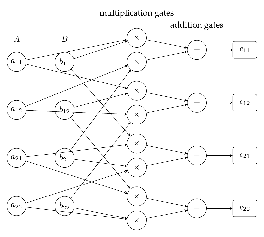
An arithmetic circuit for 2×2 matrix multiplication: eight multiplication gates and four addition gates produce four outputs.

Count the multiplication and addition gates to obtain the operation count: $12$ operations, comprising $8$ multiplications and $4$ additions. For general $n$ , the same approach uses $n^3$ multiplications and $n^2(n-1)$ additions, giving $O(n^3)$ operations. Cleverer algorithms need not follow this approach. They construct reusable intermediate results: a result is computed and charged for only once, then reused in later operations, reducing the total operation count. The classic nontrivial improvement is Strassen’s algorithm, which solves the problem in $O(n^{\log_2 7})$ operations. It is not complicated, but its circuit would be too large to draw here; interested readers can look it up. In short, this is the matrix multiplication problem under discussion.

This measure is called arithmetic complexity. You might think it is just the familiar approach of counting operations. But something more fundamental has changed. This is not the same kind of problem as one defined on a Turing machine, and its solutions are not the same thing as Turing-machine algorithms. We care only about the computation’s algebraic structure, not how numbers are encoded, stored, addressed, accessed, or represented to a given precision—or how operations are performed on an actual machine.

Arbitrary complex numbers are allowed here, which is impossible on an ordinary Turing machine, word-RAM, or real machine. That is a theorem about infinite sets, which we will not explain here. Thus the problems being handled are not the same kind as those on Turing machines; encoding and precision are not our concern. Moreover, separate treatment is permitted for each $n$ , so there need not be a single Turing-machine algorithm that handles all $n$ uniformly. This is called nonuniformity. Imagine that the methods for different $n$ have no regular pattern. To write an algorithm, we would have to use if n==1, ...; if n==2, ...; if ..., handling every $n$ as a special case. That would not be a finite program. In this sense, these “algorithms” differ from Turing-machine algorithms too.

The distinction need not always arise. We could use only well-behaved complex constants or make the circuits uniform. Under sufficiently favorable conditions, there can indeed be a corresponding Turing-machine algorithm. But there need not be one; we cannot simply assume one always exists.

Returning to OpenAI’s result, the claim is that, under the definition above, matrix multiplication requires at most $O(n^{9/4+\varepsilon})$ complex operations for any chosen $\varepsilon>0$ , with the big-O constant depending on that choice. The problem is so fundamental and important, and has been studied for so long, that OpenAI need not restate all this context in the abstract. On closer examination, however, the result rests on exactly these definitions.

FFT and…

After several examples, we arrive at the FFT. We habitually call it FFT, but strictly speaking, the problem is the DFT—discrete Fourier transform—while the fast Fourier transform, or FFT, is a family of classical algorithms for it. You do not even need to know precisely what the DFT is. It is enough to know that it is a linear transformation that takes $n$ complex numbers and produces another $n$ complex numbers; the task is to compute those outputs. OpenAI studies the so-called “unnormalized DFT,” and we will use that convention too.

In theory, we no longer need a separate section on this. The previous sections have already laid out how to analyze and understand such results. If you have absorbed their approach and methodology, you should be able to understand what these DFT papers mean yourself.

But that is “in theory.” The DFT world is astonishingly deep and bewildering, so we will still walk through it together as a practice run. We cannot cover the whole field, so we will follow OpenAI’s preprint An explicit power saving for the exact discrete Fourier transform, seeking answers to these questions:

How should we state and understand OpenAI’s result?
What does it improve on or break through? Which “parallel” results remain unaffected? In particular, how does it relate to algorithms running on actual machines?

Question time: what should we do now to understand the result?

Read the abstract. Of course.

Here it is:

We give a deterministic algorithm that computes the discrete Fourier transform at every length n in $O(n(\log n)^{1-10^{-13}})$ operations. The model uses exact complex arithmetic, unrestricted coefficients, specified Fourier roots, and unit-cost logarithmic-size indexing; scalar preparation and array organization are included.
We give a deterministic algorithm to compute the DFT for any length $n$ , using $O(n(\log n)^{1-10^{-13}})$ operations. The model uses exact complex arithmetic, unrestricted coefficients, specified Fourier roots, and unit-cost logarithmic-size indexing. Scalar preparation and array organization are also counted.

That has exactly the structure we expected: an $O(n(\log n)^{1-10^{-13}})$ algorithm, on a model. But the model…what does all that mean? It looks like we need to read the paper itself to establish the meaning of these phrases.

After some reading, we can explain them as follows:

Exact complex arithmetic: precision and numerical stability are not considered. All complex arithmetic operations are exact and cost $O(1)$ .
Unrestricted coefficients: there is no upper bound on the magnitudes of complex coefficients or intermediate quantities.
Specified Fourier roots: for each $n$ , the algorithm can obtain a specified Fourier root from the model in $O(1)$ time for use in execution. We will skip a few computability details.
Unit-cost logarithmic-size indexing: the model has integer address registers and can access memory by address. If the address length is within $O(\log(n+2))$ bits, that access costs $O(1)$ .
Scalar preparation: although the model allows all complex arithmetic operations, OpenAI imposes a stricter condition on its algorithm. It prepares input-independent scalars in a preliminary stage, and the $n$ input numbers are multiplied only by these prepared scalars. Operations in the preparation stage are charged according to the rules above: they are “included.”
Array organization costs are also included: this is not a new requirement, merely an accompanying reminder.

Feeling a little confused or exasperated? This is not a classical, standard model. OpenAI defines it itself, hence the many details. In fact, I have omitted a small portion to keep things simpler.

Only now can we state the direct result, as the paper does in Theorem 1.1: in the model above, a deterministic algorithm solves the DFT problem with complexity $O(n(\log n)^{1-10^{-13}})$ . Spelling it out would require all the detail above. In any case, “in the model above” is indispensable. In a model that supplies no roots of unity, or does not allow this kind of random access, the algorithm might not work. Conversely, if preparation were free or more and faster operations were allowed, it might run faster. At this point I surely need not say it yet again: complexity rests on a computational model.

← But you just said it again (・へ・)

You might now wonder: if the result relies on such a specialized model, why does it matter? To answer that, we need to compare it with existing DFT results.

In the classical “unrestricted linear circuit model,” the previous best result required $O(n\log n)$ operations. Does OpenAI’s $O(n(\log n)^{1-10^{-13}})$ improve on it? We must compare the power of the two models.

Roughly, the unrestricted linear circuit model means: constants are unbounded, corresponding to item 2 above; inputs undergo only linear operations, meaning addition and subtraction are allowed, but multiplication must be by scalars, corresponding to item 5. Although OpenAI’s model permits general complex multiplication, its algorithm deliberately multiplies inputs only by prepared scalars. Complexity counts only arithmetic operations, which are exact complex operations, corresponding to item 1. Constants may be chosen arbitrarily, so they of course include the Fourier roots in item 3.

For the way this algorithm operates, OpenAI’s model therefore imposes more requirements than the unrestricted linear circuit model. It also charges for memory access. Random access may cost $O(1)$ , but the circuit model does not charge for memory access at all; it has no notion of memory. An algorithm in OpenAI’s model can consequently be transferred directly to the unrestricted linear circuit model: make its prepared constants circuit constants, turn subsequent operations into gates, and replace indexing and memory access with wires. Complexity can only decrease, not increase. This also shows that, complicated as OpenAI’s model looks, many of its features restrict the algorithm rather than make its life easier, strengthening the result.

Thus, if the paper achieves $O(n(\log n)^{1-10^{-13}})$ in OpenAI’s model, it also achieves $O(n(\log n)^{1-10^{-13}})$ in the unrestricted linear circuit model. The models differ, but we reached this conclusion by comparing their relative power. That is the main breakthrough: the $O(n\log n)$ upper bound had not improved for a very, very long time.

On the other hand, an “unrestricted” linear circuit model has restricted counterparts, such as the bounded-coefficient linear circuit model, which requires coefficients to have a bound independent of $n$ . Can OpenAI’s result be transferred there too?

Naturally, no. Item 2 explicitly states that OpenAI does not require bounded coefficients. In fact, such a transfer is impossible: in 1973, Morgenstern proved an $\Omega(n\log n)$ lower bound for the DFT in the bounded-coefficient linear circuit model. This also tells us that OpenAI’s algorithm must use unbounded constants. Having read this far, you should no longer be puzzled by how the same problem can have both an $\Omega(n\log n)$ result and an $o(n\log n)$ result.

There are many other DFT models, but we do not have space to introduce them. Instead, let us use the remaining space to answer a question you may care about: what does OpenAI’s result mean for “real-world” DFT computation? Which is the “real” model—the unrestricted linear circuit model, the bounded-coefficient linear circuit model, or OpenAI’s? The answer is none of them.

All these models primarily concern the number of complex arithmetic operations and therefore assume exact complex arithmetic. In reality, how complex numbers are stored and how much precision they have cannot be ignored.

Ignoring precision is not an oversight in these models; it is deliberate. They try to set aside other difficulties, such as complex-number representation and numerical precision, to isolate the arithmetic question: how many operations are needed to implement the DFT as a linear transformation? That is only one aspect of the DFT’s difficulty. Others include numerical stability, costs on particular machines, parallel-computation costs, and costs in special cases, each giving rise to other research.

Not every result makes the DFT faster in practice, but together these results deepen our understanding of it. The same goes for other problems. Classical problems are often not single, indivisible objects, and complexity research does not advance along one linear axis. It proceeds from many angles, and even the angles themselves must sometimes be discovered. That is part of both the richness and the “confusion” of theoretical computer science.

Accounts of research that omit computational models entirely present complexity research as if it were a race to break a record. Yet even races differ in distance and conditions; some are relays, others involve hurdles. Such accounts may be effective publicity, but they are inadequate as explanations. They amount to not yet understanding the result.

This article may look like a tour of computational models, but its purpose is not to explain a few particular models. It is to teach you how to approach them. There are far too many models to cover them all. Knowing that they exist, and knowing a better way to understand complexity results, gives you a more appropriate method for approaching future results and studying problems that interest you.