Author: I Am Zhang Yixian
Author’s Zhihu profile: Thinker

Variational Inference

The basic idea is this: in probabilistic models, we often need to approximate probability distributions that are difficult to calculate. Inference about any unknown quantity can be regarded as posterior-probability inference, because Bayes’ theorem can be used to construct it:

$p(x) = \sum p(x|z)p(z)$

For large datasets, Markov chain Monte Carlo methods are too slow, so we need variational inference.

We frequently encounter two kinds of variables here: real data, $x$ , and latent data, $z$ .

The resulting inference problem is to determine the posterior conditional probability distribution $p(z|x)$ of the input data. Using the ELBO method, we hope to find a concrete distribution $q(z)$ that can approximate and replace the true posterior distribution $p(z|x)$ .

We therefore need to optimize their KL divergence:

$q^*(z) = argmin_{q(z)∈Q}KL(q(z)||p(z|x))$

The KL divergence can be rewritten further. All expectations below are with respect to $q(z)$ :

$KL(q(z)||p(z|x)) =E(\log q(z)) - E(\log p(z|x))\\ =E(\log q(z)) - E(\log p(x,z)) + \log p(x)$

We can therefore define the evidence lower bound, or ELBO:

$ELBO(q) = E(\log p(z,x)) - E(\log q(z))$

The $q(z)$ above can of course be replaced by $q(z|x)$ ; the equation then needs only a small adjustment.

Whether in a VAE, GAN, or NF, one inequality is always especially important:

Make $p_\theta(z|x)$ and $q_\phi(z|x)$ as close as possible
$D_{KL}(q_\phi(z|x)||p_\theta(z|x)) = \log(p_\theta(x)) - \sum_zq_{\phi}(z|x)\log(\frac{p_{\theta}(x,z)}{q_{\phi}(z|x)}) \\=\log(p_\theta(x)) - L(\theta,\phi;x)$
This equation seeks to make $D_{KL}$ as close to 0 as possible, which means making the two distributions as close as possible. Continuing the transformation gives:
$L(\theta,\phi;x) = E_{q_{\phi}(z|x)}[\log(p_{\theta}(x|z))] - D_{KL}(q_{\phi}(z|x)||p_{\theta}(z))$
Combining the two equations gives:
$\log(p_\theta(x)) - D_{KL}(q_\phi(z|x)||p_\theta(z|x)) = E_{q_{\phi}(z|x)}[\log(p_{\theta}(x|z))] - D_{KL}(q_{\phi}(z|x)||p_{\theta}(z))$
Our objective is to make $D_{KL}(q_\phi(z|x)||p_\theta(z|x))$ as close to 0 as possible, so we obtain the equation from the paper:
$\log(p_\theta(x)) ≥ E_{q_{\phi}(z|x)}[\log(p_{\theta}(x|z))] - D_{KL}(q_{\phi}(z|x)||p_{\theta}(z)) = -F (x)$
The formula above captures the key idea of variational inference. Here, $F$ is called the ELBO bound.

VAE (Variational Autoencoder)

A VAE seeks to make the $ELBO$ derived above as large as possible. It introduces SGVB and the reparameterization method.

The VAE network architecture is shown below:

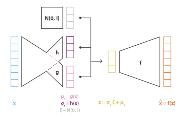
Put simply, it takes real data $x$ as input and uses the generative networks $h,g$ to produce the desired $\mu_x,\sigma_x$ :

$\mu_x = g(x) \\ \sigma_x = h(x)$

It then introduces Gaussian noise $N(0,1)$ and combines the two to construct the latent variable $z$ —the reparameterization trick, which makes backpropagation possible:

$z = \sigma_x \zeta + \mu_x$

The decoder then decodes $z$ into $\hat{x}$ :

$\hat{x} = f(z)$

Note that when training a VAE, we must ensure that $z$ follows a normal distribution. This is a major difference between a VAE and an AE: it gives the latent space a degree of regularity—continuity and completeness.

The VAE loss function is:

$L(\theta,\phi;x) = ELBO \\= E_{q_{\phi}(z|x)}[\log(p_{\theta}(x|z))] - D_{KL}(q_{\phi}(z|x)||p_{\theta}(z))$

The first term can be understood as reconstruction loss, and the second as regularization loss.

Applying maximum likelihood to the first term gives:

$(f^*,g^*,h^*) = argmax_{(f,g,h)∈F\times G \times H} (E_{z ~ q_x}(-\frac{||x-f(z)||^2}{2c}) - KL(q_x(z)||p(z)))$

How do we handle the second term? We can integrate it directly:

$- D_{KL}(q_{\phi}(z|x)||p_{\theta}(z)) = \int q_{\theta}(z)(\log p_{\theta}(z)-\log q_{\theta}(z))dz \\ = \frac{1}{2}\sum_{j=1}^J (1+\log((\sigma_j)^2)-\mu_j^2-\sigma_j^2)$

(Note that because we want the distribution of $z$ to be as close as possible to $N(0,1)$ , the mean of the distribution of $z$ is 0 and its variance is 1. For $q_{\phi}(z|x)$ , the distribution is $N(\mu,\sigma)$ .)

The second term means making $q_{\phi}(z|x)$ approach $N(0,1)$ as closely as possible. The first term is the MSE between the generated $\hat{x}$ and $x$ ; this is the term that also appears in an AE. The second is equivalent to a regularization term.

To generate a completely new image, sample $z$ directly and feed it into the decoder network. The output will be a new image.

GAN (Adversarial Learning)

A GAN consists of a generator network G and a discriminator network D:

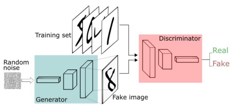
A GAN can be understood as using the cross-entropy formula to determine the similarity between distributions:

$H(p,q)=-\sum_{i}{p_i \log q_i}$

This resembles a binary-classification problem. The data either comes from the real dataset or is produced by randomly generating noise and passing it through the generator. The discriminator must then decide whether it is real or fake:

The discriminator says only “right” or “wrong.” It is a binary-classification network.

Suppose [Formula] is the distribution of correct samples. The corresponding is then the distribution of generated samples. represents the discriminator, so represents the probability that it classifies a sample as correct, while corresponds to the probability that it classifies a sample as incorrect.

Implementing this with cross-entropy gives:

Let the sample generated by the generator be $\hat{x}$ ~ $G(z)$ , where $z$ follows the distribution of the noise fed into the generator. $x$ is a real sample point.

Extending this to infinity, we rewrite it in integral form.

Here is the formal procedure:

We first fix G—that is, choose an arbitrary G—and then seek $V(G,D)$ :

$V(G,D) = \int _\infin p_{data}(x)\log D(x) dx + \int _\infin p_z(z) \log (1-D(g(z))) dz \\ = \int _\infin (p_{data}(x)\log(D(x)) + p_g(x)log(1-D(x)) )dx$

Differentiating the expression inside the integral gives the maximum $V(G,D)$ , which is the point at which $D$ performs best:

At this point:

$D^*(x) = \frac{p_{data}(x)}{p_{data}(x)+p_g(x)}$

That is:

$V(G,D) = E_{x->p_{data}}[ \frac{p_{data}(x)}{p_{data}(x)+p_g(x)}]+E_{x->p_{g}}[ \frac{p_{data}(x)}{p_{data}(x)+p_g(x)}]$

We must then keep training the generator network so as to minimize $\max_D V(G,D) = V(G,D^*)$ : $C(G) = \min_G V(G,D^*)$ .

Thus, when $p_g = p_{data} = 1/2$ —the Nash equilibrium, at which point it can no longer tell which is which—we obtain the minimum:

$\min_G\max_D V(G,D) = \min_G V(G,D^*) = -\log 4$

Substituting their minimum values and rewriting gives:

$C(G) = -log(4) + KL(p_{data}||\frac{p_{data}+p_g}{2})+ KL(p_{g}||\frac{p_{data}+p_g}{2}) \\= -log(4)+2JSD(p_{data}||p_g)$

When JSD is 0, $p_{data}$ and $p_g$ are considered equal and can no longer be distinguished from one another. At this point, C* = -log4.

NF (Normalizing Flow)

A normalizing flow is another kind of generative network, based on a change-of-variables theorem.

Suppose the generative network is still G, $z$ is a standard normal distribution—the latent variable—and x is real data.

$Z->Generator...->x$

We therefore want the distribution of the generated x to be as close as possible to the original distribution of x.

Suppose $\{x^1,x^2,...,x^m\}$ is a sample from $p_{data}(x)$ .

We want $p_G(x)$ and $p_{data}(x)$ to be as close as possible, giving the target:

$G^* =argmax_G \sum_{i=1}^m \log P_G (x^i) \\≈ argmin_G KL (p_{data}(x)||p_G(x))$

Several mathematical formulas matter here: the volume after a linear transformation equals the determinant of the transformation matrix.

[Formula]

In other words, the determinant can be regarded as the local linear rate of volume change under the transformation [Formula] .

The input and output sizes of an NF must be the same. This distinguishes it from the other two, which accept arbitrary inputs.

Now suppose that it consists of a series of flow networks.

We modify the original network accordingly:

$\log p_K (x^i) = \log \pi(z^i) +\sum_{h=1}^K \log|det(J_{G_K^{-1}})|$

We seek the maximum value of the left-hand side—that is, the maximum log likelihood.

To calculate it, we can consider the process in reverse and feed x through the $G^{-1}$ network to generate z.

Because the expression above is too computationally expensive, we need the following treatment:

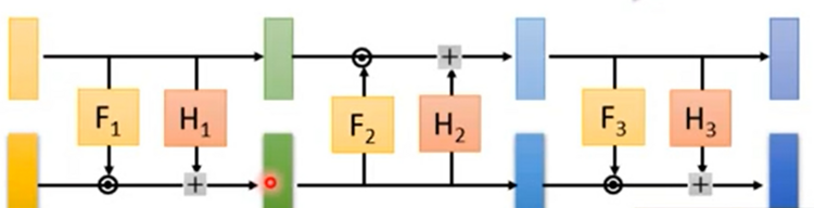
1. Coupling Layer: – > used in NICE and Real NVP

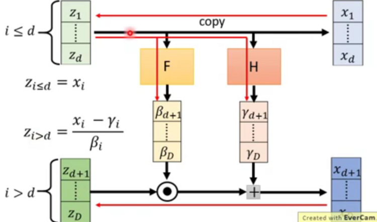
It sends the first 1:d dimensions directly from z to x. For the remaining d+1:D dimensions, the earlier data passes through the F and H networks to obtain $\beta_{d+1:D}$ and $\gamma_{d+1:D}$ , followed by a linear combination:

$x_{d+1:D} = \beta_{d+1:D} \times z_{d+1:D} + \gamma_{d+1:D}$

After the coupling layer, the Jacobian matrix becomes a triangular matrix:

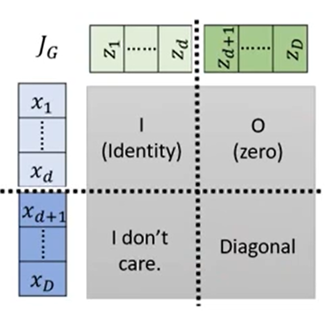
The upper portion is copied directly, so it is 1:1, while the values along the lower-right diagonal (D>i>d+1) are the $\beta_i$ values.

The determinant of the Jacobian can therefore be written as:

$det(J_G) = 1\times 1 \times ...\times 1\times \beta_{d+1}\times ...\times \beta_{D}$

But if every network is processed this way, would the first d terms not remain unchanged?

They must therefore be processed in an interleaved manner. Each network randomly selects d terms, and the size of d must also vary. Only then will stacking the networks have an effect.

1x1 Convolution

In addition to coupling layers, we can use a 1x1 convolution. This was proposed in GLOW and works especially well.

Suppose we are processing an image with three channels—the R, G, and B channels. The 1x1 convolution uses a 3x3 matrix $W$ :

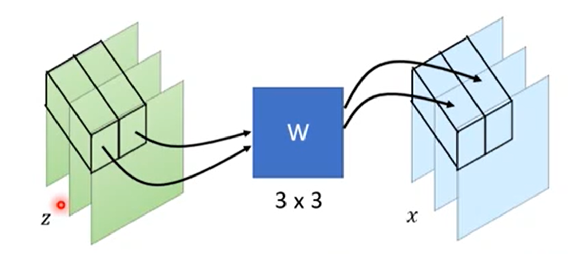
The size does not change after the 1x1 convolution, and this $W$ matrix is in fact $det(J_G)$ :

$x = f(z) =W\times z$

\begin{equation} % begin mathematical environment J_f = \left( % left parenthesis \begin{array}{ccc} % the matrix has three centered columns w_{11} & w_{12} & w_{13}\\ % first-row elements w_{21} & w_{22} & w_{23}\\ % second-row elements w_{31} & w_{32} & w_{33}\\ \end{array} \right) = W % right parenthesis \end{equation}

As long as W is easy to solve, the result is easy to calculate:

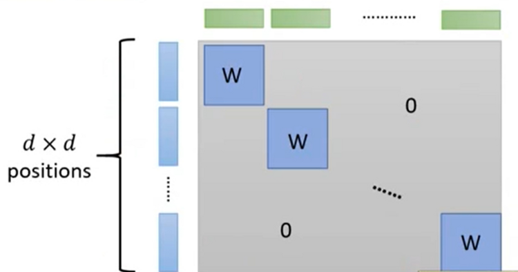
The result is therefore the product of the W matrices on the diagonal:

$(det(W))^{d\times d}$

Substituting into the formula:

$\log p_K (x^i) = \log \pi(z^i) +\sum_{h=1}^K \log|(det(W))^{d\times d}|$

This simplifies the complex computation.

References:
[1] Hung-yi Lee, Machine Learning
[2] Su Jianlin

Variational Inference and Generative Models

Variational Inference

VAE (Variational Autoencoder)

GAN (Adversarial Learning)

NF (Normalizing Flow)