Author: Zhang Yixian
Reviewer: Shiguang

Introduction

Spatiotemporal data are both complex and diverse. Analyzing them can have a major impact on weather forecasting (as with Huawei’s Pangu model), predictions of geological variation and sunspot activity, traffic-light scheduling, bike-sharing deployment, and many other tasks. Their complexity stems from temporal and spatial variation as well as spatial heterogeneity. Their distributions can also be highly extreme, with large numbers of zero values and pronounced long tails.

This article introduces a method that incorporates the Tweedie distribution and the zero-inflated negative binomial distribution to capture zero inflation and long-tail effects in complex spatiotemporal data, then combines them with a spatiotemporal graph neural network to quantify predictive uncertainty.

01 Overview

1.1 Uncertainty Quantification

Uncertainty Quantification

Imagine entering the vast field of artificial intelligence as though stepping into an unfamiliar forest, filled with the mysteries of machine intelligence and cutting-edge technology. One concept in this rapidly developing field deserves particularly close attention: uncertainty quantification. Suppose you are teaching a computer to recognize animals such as dogs, cats, and elephants. When it encounters a completely new image, it must do more than make a classification: it should also tell us how confident it is. The absence of complete confidence is uncertainty.

When a computer model makes a prediction, how can we tell how certain it is that the prediction is correct? Model uncertainty describes the extent to which a model may make an error or produce an uncertain result. It can arise from two sources: the model may have seen only limited data, while the model’s own complexity may prevent it from making consistently accurate predictions.

First, consider uncertainty arising from the data. Just as you might struggle to identify a strange animal after seeing only a few photographs of cats and dogs, a model can be confused by wholly new data. Everything it knows comes from its training data, and applying that knowledge directly to unfamiliar situations is difficult. If you had seen only black and white dogs and suddenly encountered a blue one, you would be confused too.

A second source is uncertainty inherent in the model—the limitations of the model itself. Suppose you teach a computer to distinguish cats from dogs by looking at features such as tail length and ear shape. If you then give it a blurry image, it may be unable to decide accurately. A model cannot always draw a sensible conclusion from ambiguous clues as a person can, so insufficient information may lead it to the wrong prediction.

Researchers have developed several ways to help us interpret predictions in the presence of these uncertainties. A model can, for example, report a confidence score, effectively saying either “I am highly confident in this prediction” or “I am not very sure.” Alternatively, it can output a predictive distribution that gives the probability of every possible outcome. This is much like knowing the probability of each face of a die, which lets you reason more clearly about the result.

These methods make the uncertainty behind a model’s prediction clearer. They are like a map of an unfamiliar forest, helping us take each step with greater confidence. Uncertainty quantification is widely used in medicine, transportation, finance, and other fields, allowing predictions to inform sounder and more reliable decisions.

1.2 Spatiotemporal Graph Neural Networks

Spatiotemporal Graph Neural Network

In recent years, spatiotemporal graph neural networks have become powerful deep-learning tools for understanding and processing data with temporal and spatial relationships. Analyzing changes in urban traffic or forecasting future weather, for example, requires us to model intricate connections across both time and space. These networks provide a way to explore such data.

First, what are spatiotemporal data? They contain both temporal and spatial information, such as temperature, traffic flow, or population measured at different places and times. A spatiotemporal graph is a graph structure that represents relationships and interactions within these data. In this graph, nodes represent different places or objects, and edges represent relationships between them.

A spatiotemporal graph neural network is a deep-learning model designed specifically for spatiotemporal graph data. It combines ideas from graph neural networks and time-series forecasting to extract useful information from complex data. Such a network can capture relationships between locations while tracking patterns that change over time, improving forecasts, trend analysis, and even decision optimization.

Consider an urban traffic system. Each intersection can be treated as a node, while vehicle movements between intersections at different times define the edges. A spatiotemporal graph neural network can learn how traffic flow varies across intersections and over time, helping planners improve traffic movement and reduce congestion.

This architecture has applications in many fields. In meteorology, it can analyze observations from around the world to improve forecasts of climatic change. In medicine, it can process spatiotemporal data from medical devices for disease prediction and diagnosis. In finance, it can analyze relationships between markets to support better investment decisions.

1.3 Probabilistic Models

Data analysis often presents special cases for which conventional statistical methods are inadequate. Two common examples are long-tailed data and zero-inflated data. Both have complicated distributional properties that standard statistical models may struggle to accommodate. Probabilistic models such as the zero-inflated negative binomial distribution and the Tweedie distribution are useful in these cases.

long-tailed data contain a very large number of observations at one end of the range together with comparatively rare extreme values, which can strongly affect a model. In analyses of social-media likes or sales volumes, for example, conventional statistics such as the mean and variance may not reveal the distribution’s full character.

zero-inflated data contain far more zeros than would ordinarily be expected. In health-insurance claims data, for instance, most people may submit no claim at all, producing a large number of zero values. Conventional models may perform poorly when their assumptions do not match this reality.

Long tails and zero inflation are especially conspicuous in spatiotemporal data. Consider origin–destination (O–D) flows—the traffic volume between any two places at any given time:

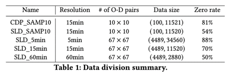
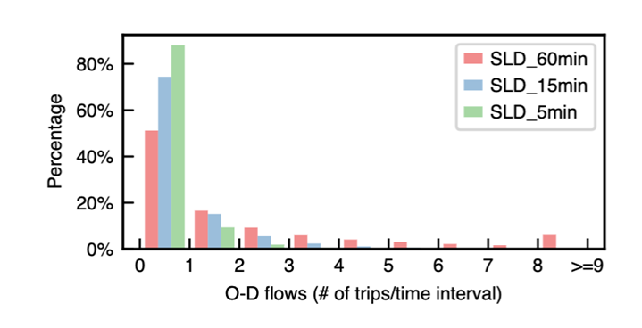
In the SLD_60min, SLD_15min, and SLD_5min datasets, zeros make up the great majority of observations, while values greater than 2 account for only a tiny fraction. This is a clear long-tail pattern.

To address these problems, the zero-inflated negative binomial distribution and the Tweedie distribution were developed.

The zero-inflated negative binomial distribution can be viewed as a combination of two components: a negative binomial distribution, a discrete distribution for count data, and a zero-inflation component that accounts for excess zeros. It is suitable when data contain both many zeros and occasional large values. The model captures the distribution more precisely, supporting better prediction and analysis.

The Tweedie distribution is a probability distribution used in generalized linear models and is suitable for long-tailed and zero-inflated data. Its broad scope allows it to handle continuous, discrete, and mixed data. Adjusting its parameters can produce a closer fit to an observed distribution.

These probabilistic models are valuable for long-tailed and zero-inflated data. They describe and explain unusual distributions more precisely while providing stronger tools for analysis and prediction. Their use in medicine, finance, the social sciences, and many other fields has broadened what data analysis can achieve.

02 Methods

This article discusses three papers published at leading conferences in data mining (SIGKDD [1] and CIKM [2]) and geographic information science (GIScience [3]). The authors are Dingyi Zhuang of MIT, Xiaowei Gao of University College London, and Xinke Jiang of Peking University.

[1] Uncertainty Quantification of Sparse Travel Demand Prediction with Spatial-Temporal Graph Neural Networks. SIGKDD 2022.

[2] Uncertainty Quantification via Spatial-Temporal Tweedie Model for Zero-inflated and Long-tail Travel Demand Prediction. CIKM 2023.

[3] Uncertainty Quantification in the Road-level Traffic Risk Prediction by Spatial-Temporal Zero-Inflated Negative Binomial Graph Neural Network (STZINB-GNN). GIScience 2023.

2.1 The Distributions

Negative Binomial Distribution

The negative binomial distribution is a discrete probability distribution describing the number of independent failures observed before a fixed number of successes occurs in repeated trials. It is commonly used when the number of trials is not fixed—for example, when a coin is tossed until a specified number of heads has appeared.

Unlike the binomial distribution, which describes the number of successes in a fixed number of trials, the negative binomial distribution concerns the number of trials needed to obtain a fixed number of successes. It has many practical uses: in finance it can describe failures before a successful investment, and in biology it can model unsuccessful attempts before an experiment succeeds. It provides a mathematical tool for understanding the probability distributions of many random events.

A negative binomial experiment has the following conditions: it consists of a sequence of independent trials, each trial has either a successful or unsuccessful outcome, the probability of success is constant, and the experiment continues until n unsuccessful outcomes have occurred, where n is a positive integer. In our spatiotemporal setting, a nonzero observation is treated as a success and a zero as a failure.

Its probability distribution is:

Here n and p are model parameters representing the number of successes and the probability of failure in a single trial, respectively.

Zero-Inflated Negative Binomial Distribution

Real-world data, however, often contain many zero observations. This excess of zeros makes the parameters of a negative binomial distribution harder to learn. A new parameter, $\pi$ , is therefore introduced to learn the zero-inflation rate, yielding the zero-inflated negative binomial distribution.

The zero-inflated negative binomial distribution (abbreviated ZINB) is a probability distribution for datasets with large numbers of zeros that also retains the properties of the negative binomial distribution.

Real-world data often contain many zeros for specific reasons. In a dataset of social-media likes, for example, many posts may receive no likes at all. A conventional negative binomial distribution may perform poorly because it cannot adequately capture this excess-zero feature.

The ZINB distribution was introduced to handle this excess-zero problem more effectively. It combines one component for zeros with another for nonzero values. More specifically, it adds a parameter $\pi$ that represents the degree of zero inflation. During data generation, a zero is produced with probability $\pi$ , while a nonzero value follows a negative binomial distribution with probability $1-\pi$ . This allows ZINB to represent data with excess zeros more accurately and makes it more suitable for modeling and analysis.

Its probability distribution is:

This expression adds a weight for zero values to the negative binomial distribution. Here pi is the zero-inflation coefficient.

ZINB is used in many fields, especially for datasets with many zeros, such as social-media and medical data. Its zero-inflation parameter helps us understand and explain these unusual datasets and provides a more accurate analytical tool.

Tweedie Distribution

The negative binomial distribution accounts for zeros to some extent but is unsuitable when zeros are extremely abundant. Introducing $\pi$ weights the zero values and improves model robustness. Excess zeros are also associated with a long tail, so the long-tail effect must be modeled as well. This leads to the Tweedie distribution.

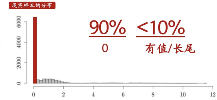
Figure source: Zhihu user “Always Learning, Always Happy”

The Tweedie distribution is a probability distribution used in generalized linear models to model and analyze positive-valued data with complex distributional properties. It can describe continuous, discrete, and mixed data. The Tweedie family includes several familiar special cases, among them the normal, gamma, and Poisson distributions. This flexibility lets it adapt to different distributions without requiring a separate model for every case. Its parameterization depends principally on a power parameter and a dispersion parameter. The power parameter determines the distribution’s shape, while the dispersion parameter controls its spread. Choosing them appropriately allows a Tweedie distribution to fit many kinds of data, including long-tailed and zero-inflated data.

The probability density function of the Tweedie distribution is:

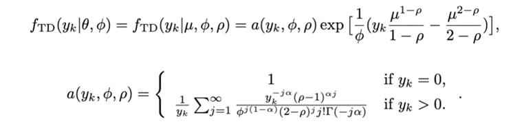
There are three parameters: the dispersion coefficient $\phi$ , the power parameter $\rho$ , and the model mean $\mu$ .

In practice, the Tweedie distribution is widely used for diverse and complex datasets, including insurance claims, financial time series, and ecological observations. It captures and explains their distributional properties more effectively, supporting more precise analysis, modeling, and prediction.

In summary, to model both the data and their uncertainty at a particular location and time in a spatiotemporal graph, we use a two-parameter model (NB) and three-parameter models (ZINB and Tweedie) to quantify model uncertainty.

2.2 Spatiotemporal Graph Neural Networks

Modeling the parameters of each distribution is difficult. For spatiotemporal data, we can use a spatiotemporal graph neural network.

To learn these parameters, we use a spatiotemporal graph neural network (STGNN). Its design resembles solving a puzzle: a temporal encoder and a spatial encoder work together to learn the parameter values.

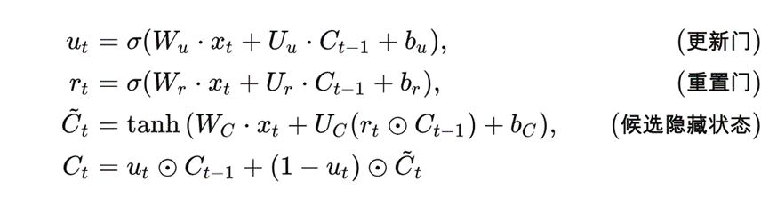
More specifically, the temporal encoder uses a gated recurrent unit (GRU) to process temporal information in the data. Its operation is loosely inspired by certain processes in the human brain.

GRU equations

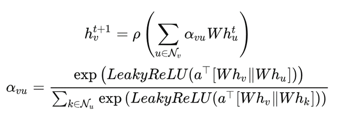
The spatial encoder uses a graph attention network (GAT), which establishes connections between observations and helps us understand their relationships.

GAT equations

The STGNN architecture is shown below:

Figure source: Zhihu user Lucia

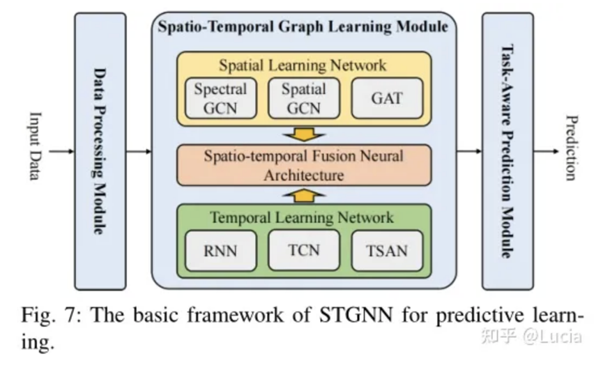
This specialized spatiotemporal graph neural network learns the parameters of the data model—whether there are two, three, or more—and uses them to construct the output distribution. The result supports stronger analysis and more reliable predictions. Like solving a puzzle, continually refining the network makes the analysis more accurate and useful.

2.3 Model-Training Objective

The authors use maximum likelihood to guide model training.

Maximum likelihood is a standard method in statistics and probability for finding the parameter values under which the observed data are most probable.

Consider a simple example. Suppose you have the outcomes of many die rolls and want to determine whether the die is fair or biased. You know it has six faces but not the probability of each face. You can use a parameter $p$ to represent those probabilities and then construct a probabilistic model.

Now suppose you have actual observations from 100 rolls. The goal is to find a value of $p$ that maximizes the probability of observing those 100 outcomes.

That is the principle of maximum likelihood. The likelihood function represents the probability of the observed data for a given parameter value. We adjust the parameter to maximize that probability—in other words, to make the observations as probable as possible under the model.

Maximum likelihood is a method for finding optimal parameters and is used in machine learning and statistical analysis. Parameters that fit the data well reveal its patterns more clearly and support more accurate predictions and decisions. The process resembles assembling a puzzle: we keep trying configurations until the model best matches reality.

ZINB Maximum-Likelihood Function

The parameters $\pi$ , $n$ , and $p$ are learned by the STGNN. Repeatedly optimizing this function trains the model.

Tweedie Maximum-Likelihood Function

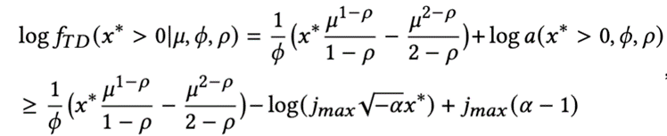
The parameters $\rho$ , $\phi$ , and $\mu$ are learned by the STGNN. Repeatedly optimizing this function trains the model.

References