How Do We Send Spacecraft to Other Planets? A Brief Guide to Motion and Orbits

Author: 丛雨
Reviewer: 时光

How many steps does it take to send a probe to Mars? In general, a probe’s journey from Earth to another planet can be divided into three stages: the rocket launches and enters Earth orbit; the spacecraft accelerates onto a new trajectory, escapes Earth’s gravity, and travels toward the target planet; and, after arrival, it either enters orbit around that planet or lands on it. The first and third stages are brief but involve many intricate steps and details, while the second occupies most of the journey. Beginning with spacecraft motion and orbital trajectories, this article introduces some basic ideas about celestial motion and orbital maneuvers.

The Three Cosmic Velocities

Let us begin with spacecraft speed.

As everyone knows, the faster an object is thrown horizontally, the farther away it lands. Once its speed reaches 7.9 km/s, it no longer falls back to the ground; under the influence of Earth’s gravity alone, it travels around Earth in uniform circular motion. This is Earth’s first cosmic velocity: the minimum initial speed needed to launch an artificial satellite and the maximum linear speed of a circular orbit around Earth.

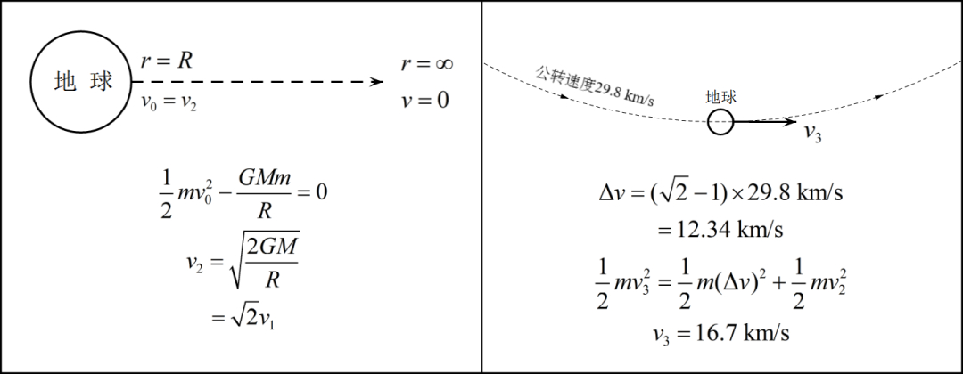
If the initial launch speed reaches approximately 11.2 km/s—Earth’s second cosmic velocity—the spacecraft can just escape Earth’s gravity completely without any further acceleration. A celestial body’s second cosmic velocity is also called its escape velocity. An unpowered object launched in any direction from the body’s surface at escape velocity gradually slows under gravity, reaching a speed of exactly $0$ at infinity. Escape velocity is $\sqrt{2}$ times the first cosmic velocity. We can calculate it from the conversion between kinetic energy and gravitational potential energy ($E_p = -GMm/r$, taking the potential energy at infinity as zero). During the escape, kinetic energy is gradually converted into gravitational potential energy until both reach $0$ at infinity.

The third cosmic velocity is the minimum initial launch speed required to escape the gravity of both Earth and the Sun. Unlike the second cosmic velocity, which may point in any direction, the third requires the spacecraft’s initial motion to follow the same direction as Earth’s revolution around the Sun. This takes advantage of Earth’s orbital velocity and reduces fuel consumption. As explained above, the Sun’s escape velocity at Earth’s orbit is $\sqrt{2}$ times the circular-orbit speed of 29.8 km/s, or about 42.1 km/s. A spacecraft therefore needs the kinetic energy corresponding to the 12.3 km/s difference between those values to escape the Sun, plus the kinetic energy corresponding to another 11.2 km/s to escape Earth. The speed corresponding to the sum of these two kinetic energies is the third cosmic velocity, 16.7 km/s.

Interplanetary spacecraft traveling between Earth and other planets plainly have destinations far enough away that they must, in a sense, overcome Earth’s gravity completely. Yet they do not leave the Sun’s gravitational domain, so their speeds usually lie between $v_2$ and $v_3$.

Deriving the second and third cosmic velocities

Orbits at Different Speeds

Next, let us consider the orbital shapes produced by different speeds and launch directions.

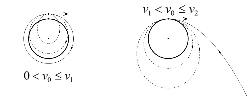
The simplest case is an object launched horizontally. At the first cosmic velocity $v_1$, its orbit is circular. If the speed is slightly greater, the object’s centripetal acceleration exceeds what gravity provides, and its orbit becomes an ellipse, with Earth’s center at one focus and the launch point at periapsis. As the initial speed rises, the ellipse grows increasingly elongated, while its apoapsis altitude, semimajor axis, and eccentricity all increase. If the object is launched at the second cosmic velocity $v_2$, the eccentricity becomes 1 and both the semimajor axis and apoapsis distance become infinite, producing an open parabolic trajectory. If the initial speed exceeds $v_2$, the spacecraft follows one branch of a hyperbola relative to Earth. Its eccentricity is greater than 1, and in celestial mechanics its semimajor axis is defined as negative.

Now consider horizontal launches slower than $v_1$. Strictly speaking, their trajectories are also ellipses. When the initial speed is very low, however, the ellipse is likewise extremely elongated and its eccentricity approaches $1$, so the path can be treated as a parabola. In this case, the launch point is the ellipse’s apoapsis, while its periapsis lies inside Earth.

Orbital shapes produced by different horizontal launch speeds

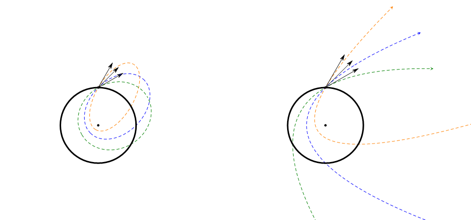
In fact, apart from the special case of a vertically upward launch, an object follows an elliptical, parabolic, or hyperbolic path when its initial speed is, respectively, less than, equal to, or greater than $v_2$, even if the launch is not horizontal. Different launch directions, however, produce different semimajor axes and eccentricities for ellipses or hyperbolas, and different focal lengths for parabolas. In these nonhorizontal cases, if we know the speed and the length of the radius vector, we can determine the orbit’s shape and semimajor axis by calculating the object’s mechanical energy. A sum of kinetic and potential energy that is less than, equal to, or greater than $0$ corresponds, respectively, to an elliptical, parabolic, or hyperbolic orbit. Because the mechanical energy of a two-body system is $E = -GMm/2a$, we can then find the semimajor axis $a$.

Orbits produced by launches at v1 and v2 in different directions

Orbital Maneuvers and Hohmann Transfers

Finally, let us turn to orbital maneuvers. Real trajectory changes and mission designs are necessarily extremely complex, so we will cover only a few basic principles and ideas.

Consider a spacecraft or satellite circling Earth in a low circular orbit. It fires its engine and accelerates in its direction of travel. Its speed is now greater than the circular-orbit speed at that point, and its centripetal acceleration exceeds what circular motion requires. The orbit becomes an ellipse whose periapsis is the point of acceleration, just like the surface-launch case discussed above in which the speed lies between $v_1$ and $v_2$. When the spacecraft reaches apoapsis, it accelerates by the appropriate amount once more in its direction of travel, bringing its speed exactly to the circular-orbit speed at that distance. It has now transferred into a circular orbit with a larger radius and a greater altitude than the original one. This is the basic idea behind an orbital maneuver. To lower an orbit, simply reverse the process: decelerate into an elliptical orbit, then decelerate again at periapsis.

Diagram of a satellite changing orbit

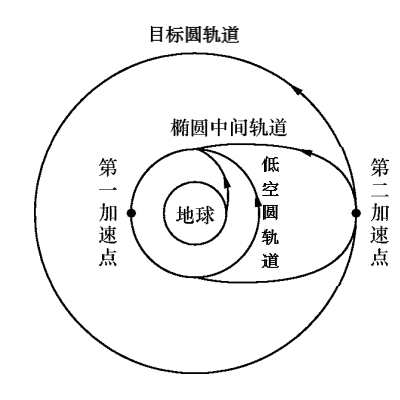
Of course, the new orbit need not be circular. A single brief engine burn may not release enough energy to reach the target altitude. The satellite can wait until it completes an orbit and returns to its starting point before firing again, or it can perform a series of maneuvers, accelerating each time it reaches apoapsis. Its successive trajectories are then nested ellipses of different sizes. Acceleration and deceleration are not limited to apoapsis and periapsis, respectively, but using the target altitude as apoapsis requires the least fuel. A greater initial speed requires more initial kinetic energy, so using exactly the speed needed to reach a specified point naturally saves energy.

The same tangential-transfer principle extends to travel between planets. A trajectory that takes a point on an inner planet’s orbit as its perihelion and a point on an outer planet’s orbit as its aphelion, while remaining tangent to both planetary orbits, is called a Hohmann transfer orbit. It is the most energy-efficient route for interplanetary travel. To fly to an outer planet, a spacecraft accelerates in the direction of Earth’s orbital motion, then accelerates again near the target planet to catch up with it. To travel to an inner planet, it decelerates opposite the direction of revolution, then decelerates again near the target planet to remain there. Because the planets of the Solar System are constantly moving and their positions relative to Earth continually change, the best launch opportunities for an interplanetary spacecraft recur periodically. That interval is the synodic period of Earth and the target planet.

A Hohmann transfer orbit from Earth to Mars

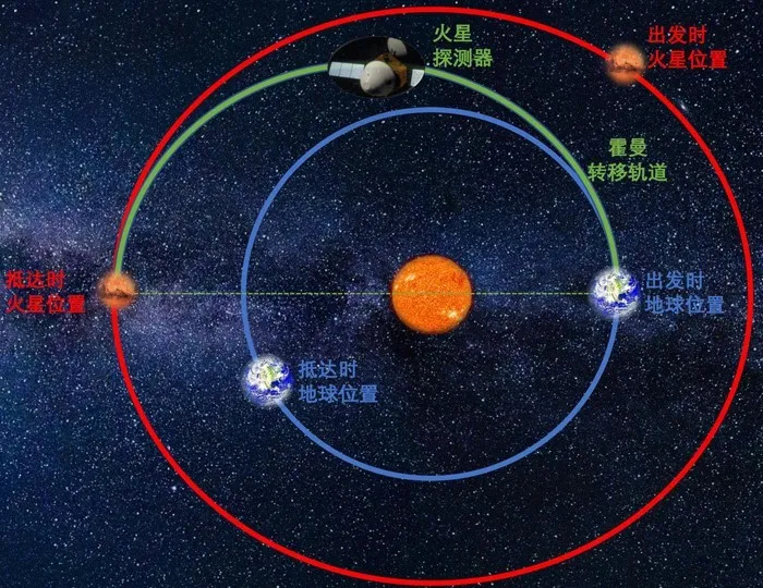
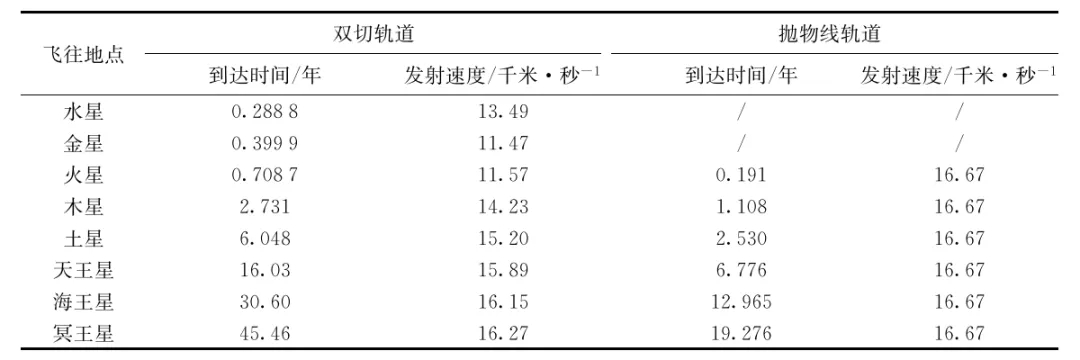
Because a Hohmann transfer follows a long route at low speed, it takes a great deal of time. In some situations, saving fuel at such a cost in time may not be worthwhile. A parabolic trajectory can be used instead. This requires reaching the Sun’s escape velocity at Earth’s orbit—the initial velocity relative to Earth is, of course, 16.7 km/s—and spending more fuel on acceleration and deceleration during departure and arrival. The table below lists the travel times to the planets. Compared with a bitangential Hohmann transfer orbit, a parabolic trajectory is indeed much faster.

Travel times for Hohmann and parabolic trajectories

Finally, remember that the planets do not move in perfect circles and that their orbital inclinations differ. An interplanetary spacecraft’s route must also account for gravitational perturbations from planets other than its target, the effects of solar eruptions, and even the safety of crossing the asteroid belt. Real trajectory design clearly cannot be explained in a few sentences. This article offers only a brief introduction—a starting point for further study.