An Introduction to the Gibbs Phenomenon
Author: phy Dongxi
First-year students taking Calculus II are probably wrestling with Fourier series by now, and many are no doubt complaining about the complicated integrals. Anyone with plotting software, however, has probably tried using trigonometric functions to approximate a periodic function. Careful observers may have noticed a curious effect: when a periodic function with a discontinuity is expanded as a Fourier series and then reconstructed from finitely many terms, adding more terms moves the peaks of the reconstructed waveform closer to the discontinuity. As the number of terms grows, the overshoot approaches a constant value of about 9% of the total jump. This is the Gibbs phenomenon.
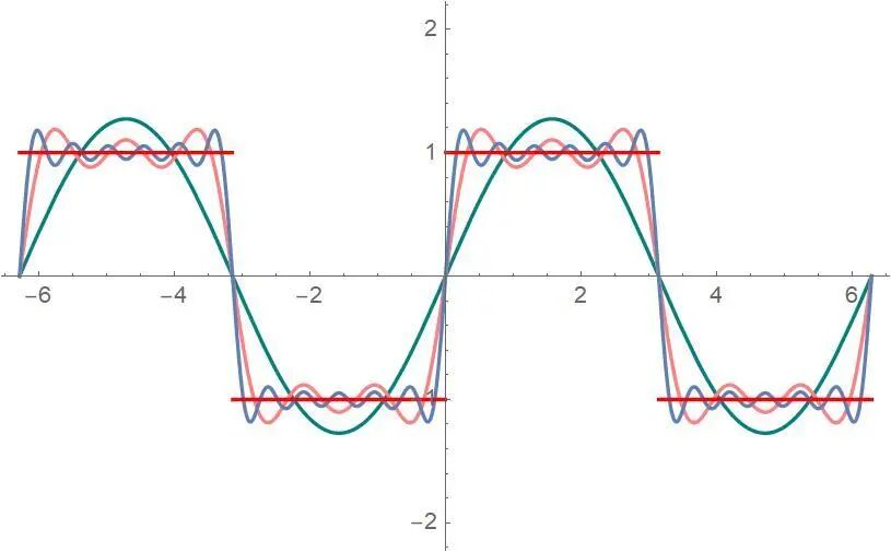
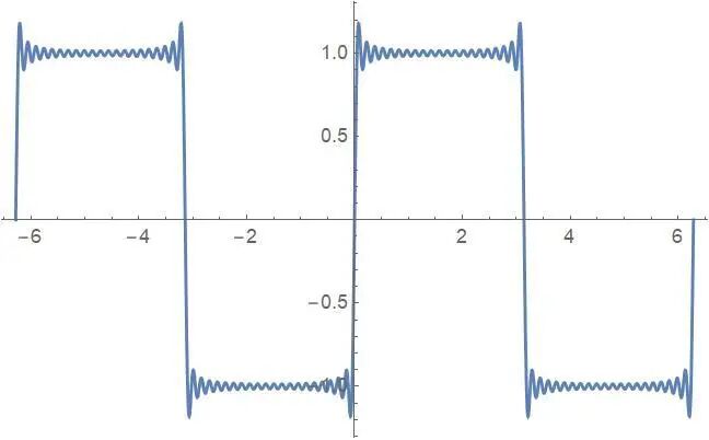
Adding more terms does not reduce the overshoot; it only moves the peak closer to the discontinuity. Here is a somewhat informal derivation:
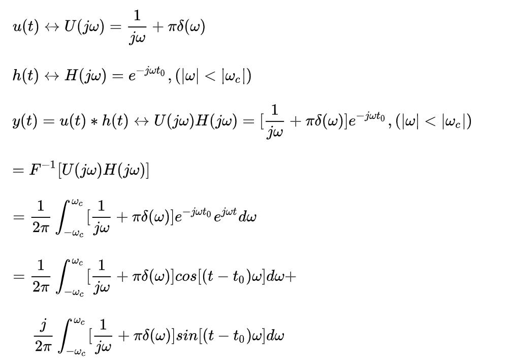
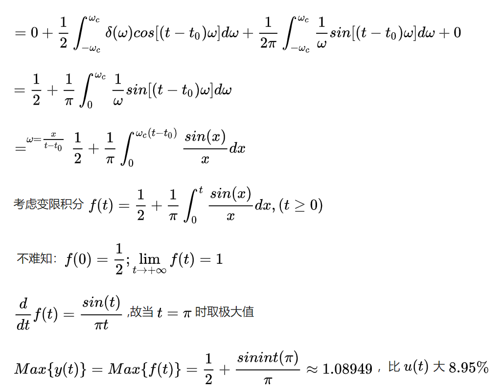
For convenience, start with a square wave and let its period grow. In the limit, it becomes a step function whose value is 0 for a negative argument and 1 otherwise. This function is clearly not periodic, or equivalently, its period is infinite. How can a nonperiodic function have a Fourier series? As the period approaches infinity, the spacing between adjacent frequencies, the fundamental frequency 1/T, approaches zero and the spectrum becomes continuous. Following this limit further leads to the definition of the Fourier transform. If a function has a Fourier transform, sampling its frequency domain at intervals of 1/T gives the Fourier series of its periodic extension with period T. Keeping only finitely many terms is then equivalent to applying an ideal low-pass filter: frequency components below the cutoff Wc remain, while all others are set to zero. The derivation in the figure produces the result for the Gibbs phenomenon.
 爱发电(点击图片跳转)